how to delete filtered rows in excel

Excel provides a wide range of functionality, a lot of which most users are not even aware of. One of its most fascinating features is the versatility of its Filters.

Excel filters provide a great way for you to view only the data that you need while keeping non-relevant rows hidden.

This way, you get to focus on specific data, without the clutter. While operating one of these filters, you might feel the need to delete some of these 'non-relevant' rows, maybe because you don't need them anymore.

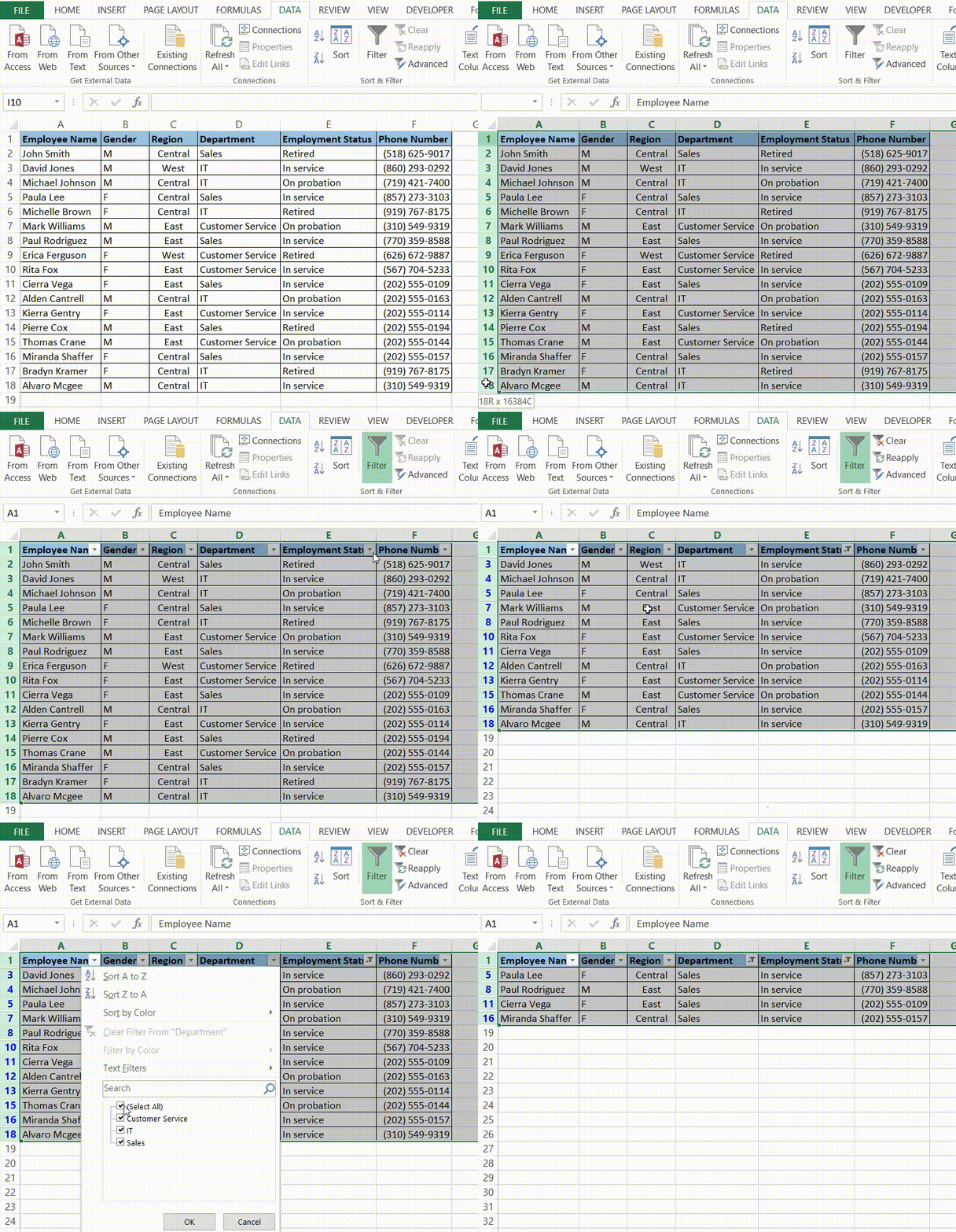
For example, in the dataset below, we have data about a company's employees. As you can see, some of these employees are retired, some are still in service, while few of them are on probation.

Dataset from which filtered rows need to be deleted

You might not need the information about retired employees anymore. So, you might want to delete rows containing information about retired employees.

The problem is, you don't want to manually search every row to find the ones with Employment Status= "Retired". That beats the whole purpose of using computerized spreadsheets, doesn't it?

The best solution is to use filters to help you in the process. In this article, we will show you how to delete filtered rows in Excel.

We will show you how to delete both the visible rows after you apply a filter, as well as the invisible rows.

If you like to code and would like to speed up your Excel processes using VBA code, we have a few snippets of code that you can use too.

Click here to download the example file and follow along

Deleting Filtered Rows that are Visible

For the above problem, you can filter the rows that you don't need and then delete these rows. Here's how:

Select the entire working area of your dataset.
From the Data tab, select the Filter button (under the 'Sort and Filter' group).
You will notice small arrows on every cell of the header row. These are meant to help you filter your cells. You can click on any arrow to choose a filter for the corresponding column.
In this example, we want to filter out only the rows that contain the Employment status "Retired". So, select the arrow next to the Employment Status header and uncheck the boxes next to all the statuses, except "Retired". You can simply uncheck "Select All" to quickly uncheck everything and then just select "Retired".
Click OK. You will now see only the rows with Employment Status "Retired".
Select all the rows in a view, right-click and select "Delete Row" from the popup menu. This will delete all the visible rows only. Don't worry, the rest of your data is safe.
To see the rest of the data, simply click on the Filter button from the Data tab again.

You should now see all your data, without the rows containing details about Retired employees.

Dataset from which filtered rows have been deleted

Deleting Filtered Rows that are Visible using VBA

If you are comfortable with the idea of writing (or copy-pasting) some VBA code, here's a quicker way to get the above task done. We've put together a short script that you can just copy, customize, and use:

Sub DeleteVisibleRows() Dim Rng As Range Set Rng = Selection Rng.AutoFilter Field:=5, Criteria1:="Retired" Rng.Offset(1, 0).SpecialCells(xlCellTypeVisible).EntireRow.Delete ActiveSheet.AutoFilterMode = False End Sub

This code takes a selection of rows and applies the 'AutoFilter' to it according to your criteria (line 4). This makes sure that only rows that qualify the given criteria get displayed.
```
Rng.AutoFilter Field:=5, Criteria1:="Retired"
```
After this, the code checks for only those rows that are visible (barring the column headers) and deletes them (line 5).
```
Rng.Offset(1, 0).SpecialCells(xlCellTypeVisible).EntireRow.Delete
```
Finally, it removes the filters by setting the sheet's AutoFilterMode to False (line 6).
```
ActiveSheet.AutoFilterMode = False
```

Follow these steps to use the above code:

Select all the rows you need to filter (including the column headers)
From the Developer Menu Ribbon, select Visual Basic.
Once your VBA window opens, Click Insert->Module and paste the above code in the Module window.
Run this script by navigating to Developer->Macros-> DeleteVisibleRows or clicking on the green play button from the toolbar on top.

Note: You can change line 4 to fit your own filter criteria. Replace the number '5' with the number of the column you want to apply the filter to. That means if you want to apply the filter to column A, you need to change it to "1". Replace the criterion "Retired" with the Criterion you want the filter to satisfy (for deletion). Also note that if you have more than one criteria, you can repeat this line for each criterion.

Deleting Filtered Rows that are Hidden

Let us now come to a scenario where you have a more complex filter.

Say, you only want details of Sales employees who are still in service or on probation. When you have more complex filters, one would usually prefer to delete the rows that don't qualify, rather than those that do qualify.

In other words, one would prefer to delete the rows that are hidden after filtering.

Let us use the same dataset that we had used before and this time, apply two filters – one to remove rows with Employment Status= "Retired" and another to remove any row that does not contain Department= "Sales"

Here's the filtering process first:

Select the entire working area of your database
From the Data tab, select the Filter button (under the 'Sort and Filter' group).
Select the filter arrow next to the Employment Status header and uncheck the box next to "Retired".
Next, select the filter arrow next to the Department header and uncheck all boxes except "Sales".
Click OK. You will now see only the rows with Employment Status either "In service" or "on probation" and Department="Sales".

Filtered all records for sales data

Now it is time to delete the hidden rows. There are three ways to do this.

Deleting Hidden Rows using the Inspect Document feature

If you are sure you will never need to work with the hidden data again, then this method can work for you:

Make a backup copy of your workbook (just in case).
Click on File->Check for Issues.
Click on Inspect Document.
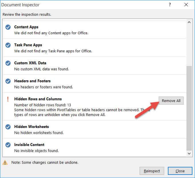
This will open the 'Document Inspector'. Click on the 'Inspect' button at the bottom of the window.
When you scroll down the list of options provided, you will see an option that says 'Hidden Rows and Columns'. It will also tell you how many hidden rows and columns are present in your worksheet.
Click on the "Remove All" button. This will permanently delete all hidden rows in your sheet.
Click 'Close'.
Go back to your sheet and remove all filters by clicking on the Filter button from the Data tab again.

You will find that even after all filters are removed, you are left with only your required rows. All other rows have been deleted.

Deleting Hidden Rows by Creating a Temporary Column

If you don't really want to bother with making backups or are worried about making permanent changes to other sheets in your worksheet, then here's another way (more of a trick) to get rid of your hidden rows:

Create a temporary column anywhere in your dataset.
Type a '0' on the first cell of this column and press the Return key.
Double click on the fill handle (on the bottom right corner) of this cell. This will copy the number '0' to the rest of the column cells.
Remove the filters (by clicking on the Filter button from the Data tab again). This will bring back all your hidden rows too.
Now you need to reverse the filter. For this, select your work area and click on the Filter button. Select the arrow next to the header of the temporary column and uncheck the checkbox next to '0'.
Select all these rows, right-click and select "Delete".
Once again remove the filters by clicking on the Filter button.

Add a helper column to delete filtered rows

You should now be left with only your required rows.

Deleting Filtered Rows that are Hidden using VBA

Once again, here's a quicker way to get the above task done. You will find below a short script that you can copy, customize, and use:

Sub KeepVisibleRows() Dim myUnion As Range Dim myRow As Range Dim Rng As Range Set Rng = Selection Rng.AutoFilter Field:=4, Criteria1:="Sales" Rng.AutoFilter Field:=5, Criteria1:="<>Retired" ForEach myRow In Rng.Rows If myRow.Hidden Then If Not myUnion IsNothingThen Set myUnion = Union(myUnion, myRow) Else Set myUnion = myRow EndIf EndIf Next myUnion.Delete ActiveSheet.AutoFilterMode = False End Sub

Follow these steps to use the above code:

Select all the rows you need to filter (including the column headers)
From the Developer Menu Ribbon, select Visual Basic.
Once your VBA window opens, Click Insert->Module and paste the above code in the Module window.
Run this script by navigating to Developer->Macros-> KeepVisibleRows or clicking on the green play button from the toolbar on top.

Here's an explanation of the code:

This code takes a selection of rows and applies the 'AutoFilter' to it according to your criteria (lines 6 and 7).
```
Rng.AutoFilter Field:=4, Criteria1:="Sales"  Rng.AutoFilter Field:=5, Criteria1:="<>Retired"
```
In line #6 we have specified that we want only the rows with Department equal to "Sales" (column 4) to be displayed.
```
Rng.AutoFilter Field:=4, Criteria1:="Sales"
```
Similarly, in line 7 we have specified that we want only the rows with Employment Status not equal to "Retired" (column 5) to be displayed (The symbol "<>" means "not equal to").
```
Rng.AutoFilter Field:=5, Criteria1:="<>Retired"
```
These two lines ensure that only the rows that satisfy both the criteria get displayed, while the others remain hidden.
After this, the code loops through each row and checks if any of them are hidden (line 9).
```
If myRow.Hidden Then
```
If so, they are grouped together into a temporary range named "myUnion". Once all the rows have been looped through, all the hidden rows will be added to myUnion.
```
Set myUnion = Union(myUnion, myRow)
```
After the looping ends, all the rows that are grouped in myUnion will get deleted (line 17). This means all the hidden rows will get deleted in one go.
```
myUnion.Delete
```
Finally, all filters will get removed by setting the sheet's AutoFilterMode to False (line 18).
```
ActiveSheet.AutoFilterMode = False
```

Note: As mentioned before, you can change lines 6 and 7 to fit your own filter criteria. If you have more than one criteria, you can repeat these lines for each criterion.

Conclusion

In this tutorial, we showed you two ways to delete the visible rows after applying filters to them and three ways to delete the hidden rows after applying filters.

We have also provided short VBA scripts to help you get the work done faster if you feel confident using scripts. We hope you found this tutorial helpful.

Do let us know in the comments if you face any issues while following any of the steps.

Other Excel tutorials you may find useful:

How to Highlight Every Other Row in Excel (Conditional Formatting & VBA)
How to Unhide All Rows in Excel with VBA
How to Set a Row to Print on Every Page in Excel
How to Delete a Sheet in Excel Using VBA
How to Paste in a Filtered Column Skipping the Hidden Cells
How to Hide Columns Based On Cell Value in Excel
How to Add a Total Row in Excel Table
How to Select Rows with Specific Text in Excel
How to Remove Duplicate Rows based on one Column in Excel?
How to Move Row to Another Sheet Based On Cell Value in Excel?

how to delete filtered rows in excel

Source: https://spreadsheetplanet.com/delete-filtered-rows-excel/#:~:text=For%20this%2C%20select%20your%20work,clicking%20on%20the%20Filter%20button.

Posted by: hixthavite.blogspot.com